When characterized under standard test conditions, the LT1213CS8 shows a ~28 MHz gain‑bandwidth product and an ~8.5 V/µs slew rate—numbers that position it for fast single‑supply precision front‑ends. Accurate interpretation of these specifications and disciplined bench measurement turn datasheet claims into reliable system guarantees. This guide focuses on the most impactful specs and practical measurement methods designers use to validate real‑world performance.
Core Insight: Designers need concise rules to map datasheet metrics to circuit behavior. Typical datasheet listings include GBW, slew, input offset, noise, PSRR, and output swing with test conditions noted. This article walks through how each spec affects closed‑loop bandwidth, transient fidelity, DC accuracy, and measurement best practices so bench results match expected system performance.
Performance Benchmarks
Optimized for fast single-supply precision
Ensures signal fidelity during large transitions
Background: What the LT1213CS8 is and why it matters
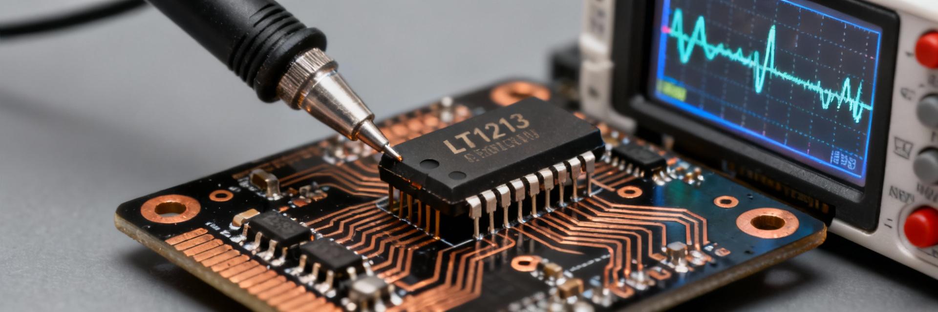
Device overview & key architecture points
The LT1213CS8 is a dual precision operational amplifier optimized for single‑supply, low‑distortion buffering and sensor front‑end tasks. Its architecture typically uses a complementary input stage with internal frequency compensation and push‑pull output capable of driving moderate loads. Those architectural choices yield the datasheet tradeoffs—moderate quiescent current, GBW around the few‑tens of MHz, and an output stage that limits headroom near supplies—so designers choose it where speed and precision must coexist on a single 5–12 V rail.
How to read the datasheet: which specs are critical for system design
Not all datasheet numbers are equally important for every design. GBW and slew define dynamic response; input offset, drift and bias set DC accuracy; PSRR and supply range determine robustness. Focus on typical versus max/min columns, and always note test conditions (VCC, temperature, RL). Flagging which values are “typical” for nominal systems and which are guaranteed limits prevents incorrect assumption of worst‑case or average behavior.
Core specifications: what they mean and how to interpret them
Frequency‑domain specs
GBW determines closed‑loop bandwidth and cascaded gain performance. With a 28 MHz GBW, a gain of +10 yields ~2.8 MHz bandwidth. For quick checks, use a small‑signal swept sine or network analyzer to extract the –3 dB point for various gains; validate that the device meets specifications under intended loading.
Time‑domain & dynamic specs
Slew rate limits large‑signal edges and affects settling for steps. The datasheet gives a typical ~8–9 V/µs measurement (20–80% step). Measure slew by applying a step that produces a sizable output excursion and record 20–80% slope to understand pulse fidelity.
Critical DC Specifications
| Specification Parameter | Key Consideration | Impact on Design |
|---|---|---|
| Input Offset & Drift | DC error sources | Dominant DC error; shifts with temperature. |
| PSRR & Supply Range | Supply dynamics | Determines noise susceptibility and headroom. |
| Quiescent Current | Power budget | Impacts thermal management in dense layouts. |
Measurement setup & best practices
Equipment & Layout
A disciplined test setup prevents measurement artifacts. Required gear includes an oscilloscope with ≥4× GBW bandwidth (≥120 MHz), a pulse generator, and low‑noise DC supplies. Use low‑capacitance probes, short ground leads, and local decoupling (0.1 µF ceramic + 10 µF bulk) close to device pins to avoid oscillation.
Step-by-Step Procedures
- • GBW & Slew: Small-signal sine sweep for -3dB point; 2V step for 20-80% slope calculation.
- • DC Offset: High-resolution DMM after thermal stabilization.
- • Noise: FFT integration over specified bandwidth (e.g., 0.1–10 MHz).
Design examples & Troubleshooting
Single‑supply 5V buffer for sensor front‑end
With a 5 V supply and unity buffer, expect bandwidth near GBW and output limited to within ~100–200 mV of rails under light loads. Choose input headroom margins, verify with a Bode sweep, and ensure input common‑mode stays inside specified range to avoid distortion.
Common anomalies and quick fixes
Oscillation often stems from long input leads or missing decoupling. Fixes include shortening leads, adding small output load resistors for stability, and using proper probe techniques. Systematic isolation of variables speeds diagnosis.
Summary Recap
- ✓ Confirm GBW and slew against closed‑loop needs—GBW defines bandwidth; compute closed‑loop bandwidth = GBW/desired gain.
- ✓ Validate DC accuracy by measuring offset and bias after thermal stabilization.
- ✓ Measure PSRR and output swing under intended supply and load to establish usable headroom.
- ✓ Use disciplined measurement setup—scope ≥4× GBW, short grounds, proper bypassing.